Basic Example

import piscola

print(f'PISCOLA version: v{piscola.__version__}')

PISCOLA version: v3.0.0

PISCOLA uses its own format for a SN file (explained SOMEWHERE ELSE) which has a similar format to that used by other codes. As an example, we have SN 03D1au (from the SNLS survey) in a file called 03D1au.dat. This file can be downloaded from the repository. To import a SN, all that needs to be done is use the call_sn() function, which receives the name of the file as an argument:

sn = piscola.call_sn('../../data/03D1au.dat')
print(sn)
print(f'Observed bands: {sn.bands}')

name: 03D1au, z: 0.50349, ra: 36.043, dec: -4.0375

Observed bands: ['Megacam_g', 'Megacam_r', 'Megacam_i', 'Megacam_z']

The sn object will contain all the necessary information, i.e. name, redshift, RA, DEC and the observed multi-colour light curves. The latter are found in sn.lcs, a Lightcurves() object, which also includes the zero-points (zp), and magnitude system (mag_sys):

sn.lcs

['Megacam_g', 'Megacam_r', 'Megacam_i', 'Megacam_z']

sn.lcs.Megacam_g

band: Megacam_g, zp: -20.846, mag_sys: AB
other attributes: times, fluxes, flux_errors, magnitudes, mag_errors

sn.lcs.Megacam_g.__dict__

{'band': 'Megacam_g',
 'times': array([52880.58, 52900.49, 52904.6 , 52908.53, 52930.39, 52934.53,
        52937.55, 52944.39, 52961.45, 52964.37, 52992.33, 52999.32]),
 'fluxes': array([-1.85848101e-20,  1.70044129e-18,  1.89317266e-18,  1.85866457e-18,
         4.68383103e-19,  3.39987304e-19,  3.07085307e-19,  1.45787510e-19,
         1.58865710e-19,  8.00752930e-20,  8.87940928e-20,  2.56975152e-21]),
 'flux_errors': array([3.93722644e-20, 9.87059915e-20, 5.70393061e-20, 5.37353399e-20,
        4.80910642e-20, 4.34563338e-20, 7.37426910e-20, 8.37463666e-20,
        7.89280825e-20, 5.21292452e-20, 6.20411439e-20, 5.51119925e-20]),
 'zp': np.float64(-20.845742237479524),
 'magnitudes': array([        nan, 23.57785366, 23.4612822 , 23.48125521, 24.97775471,
        25.32560101, 25.43611017, 26.24495696, 26.15168234, 26.89551142,
        26.78329758, 30.62952993]),
 'mag_errors': array([        nan,  0.06302403,  0.03271209,  0.03138942,  0.11147757,
         0.13877611,  0.26072595,  0.62369171,  0.53941833,  0.70681738,
         0.75861258, 23.28516396]),
 'mag_sys': 'AB'}

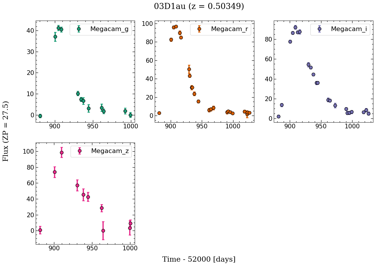
The light curves can be plotted by calling the function sn.plot_lcs():

sn.plot_lcs()

To fit the light curves one needs to use sn.fit(), where the user can decide which kernels to use. By default, PISCOLA uses Matern52 for the time axis, and ExpSquared for the wavelength axis. The wavelength axis is fitted in logarithmic space. One can also plot the fits afterwards by using sn.plot_fits(). From the fits, one gets an estimation of the epoch of rest-frame B-band peak (plotted as a vertical dashed line):

sn.fit()

sn.plot_fits()

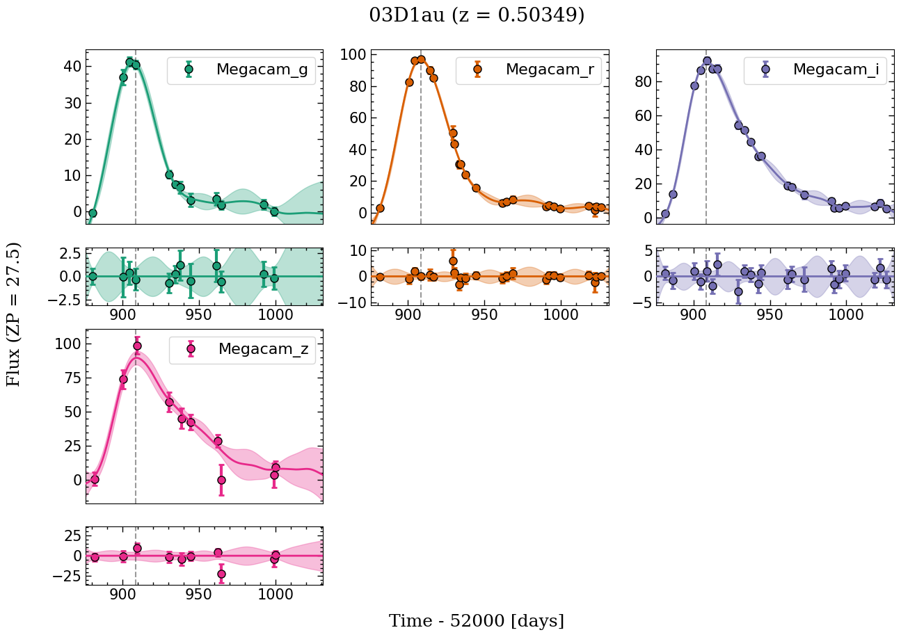
The fitting process includes: the fits of the observed light curves, Milky-Way extinction correction and redshift correction. Finally, we can check the calculated rest-frame light-curves parameters:

sn.lc_parameters

{'tmax': np.float64(52908.356),
 'tmax_err': np.float64(0.121),
 'mmax': np.float64(23.039),
 'mmax_err': np.float64(0.015),
 'dm15': np.float64(0.837),
 'dm15_err': np.float64(0.033),
 'colour': np.float64(-0.034),
 'colour_err': np.float64(0.041),
 'Bessell_B': {'tmax': np.float64(52908.356),
  'tmax_err': np.float64(0.121),
  'mmax': np.float64(23.039),
  'mmax_err': np.float64(0.015),
  'dm15': np.float64(0.837),
  'dm15_err': np.float64(0.033)},
 'Megacam_g': {'tmax': np.float64(52908.657),
  'tmax_err': np.float64(0.21),
  'mmax': np.float64(22.989),
  'mmax_err': np.float64(0.015),
  'dm15': np.float64(0.628),
  'dm15_err': np.float64(0.03)},
 'Megacam_r': {'tmax': np.float64(52909.258),
  'tmax_err': np.float64(3.053),
  'mmax': np.float64(22.932),
  'mmax_err': np.float64(0.108),
  'dm15': np.float64(0.563),
  'dm15_err': np.float64(0.176)},
 'Megacam_i': {'tmax': np.float64(52909.409),
  'tmax_err': np.float64(13.405),
  'mmax': np.float64(22.722),
  'mmax_err': np.float64(0.497),
  'dm15': np.float64(0.922),
  'dm15_err': np.float64(0.944)},
 'Megacam_z': {'tmax': np.float64(52909.409),
  'tmax_err': np.float64(20.515),
  'mmax': np.float64(22.981),
  'mmax_err': np.float64(1.173),
  'dm15': np.float64(1.099),
  'dm15_err': np.float64(2.642)}}

In Summary

To fit a supernova, simply follow these steps:

import piscola

sn = piscola.call_sn('../../data/03D1au.dat')
sn.fit()

The sn object can also be stored…

sn.save()

and later be loaded…

sn2 = piscola.load_sn('03D1au.pisco')
sn2

name: 03D1au, z: 0.50349, ra: 36.043, dec: -4.0375