Extensive Example

import piscola

print(f'PISCOLA version: v{piscola.__version__}')

PISCOLA version: v3.0.0

In this example, we will use a different SN. We will use SN 2008gp, a well-sampled low-z SN observed by the Carnegie Supernova Project (CSP).

sn = piscola.call_sn('../../data/SN2008gp.dat')
sn.plot_lcs()

PISCOLA simply fits the light curves with Gaussian Process using the sn.fit() function. This estimates the optical (B-band) peak and other parameters.

sn.fit()

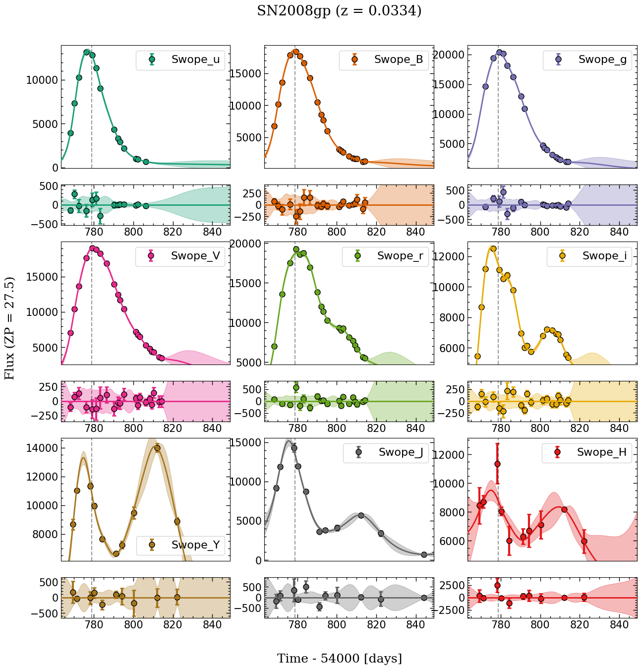
sn.plot_fits()

In this case, we see that PISCOLA does a good job fititng the optical light curves, but not so well with the near-infrared (NIR) light curves (YJH) due to the large scale difference in flux.

We can use fit_type="log" as argument to fit in log space, or fit_type="asinh" to use an inverse arcsine function, which can deal with negative values.

sn.fit(fit_type="log")

sn.plot_fits()

sn.lc_parameters

{'tmax': np.float64(54778.845),
 'tmax_err': np.float64(0.082),
 'mmax': np.float64(16.454),
 'mmax_err': np.float64(0.011),
 'dm15': np.float64(1.041),
 'dm15_err': np.float64(0.017),
 'colour': np.float64(-0.088),
 'colour_err': np.float64(0.017),
 'Bessell_B': {'tmax': np.float64(54778.845),
  'tmax_err': np.float64(0.082),
  'mmax': np.float64(16.454),
  'mmax_err': np.float64(0.011),
  'dm15': np.float64(1.041),
  'dm15_err': np.float64(0.017)},
 'Swope_u': {'tmax': np.float64(54777.295),
  'tmax_err': np.float64(0.084),
  'mmax': np.float64(16.617),
  'mmax_err': np.float64(0.026),
  'dm15': np.float64(1.423),
  'dm15_err': np.float64(0.029)},
 'Swope_B': {'tmax': np.float64(54778.949),
  'tmax_err': np.float64(0.083),
  'mmax': np.float64(16.448),
  'mmax_err': np.float64(0.011),
  'dm15': np.float64(1.047),
  'dm15_err': np.float64(0.017)},
 'Swope_g': {'tmax': np.float64(54779.259),
  'tmax_err': np.float64(0.084),
  'mmax': np.float64(16.426),
  'mmax_err': np.float64(0.011),
  'dm15': np.float64(0.849),
  'dm15_err': np.float64(0.019)},
 'Swope_V': {'tmax': np.float64(54779.879),
  'tmax_err': np.float64(0.203),
  'mmax': np.float64(16.532),
  'mmax_err': np.float64(0.012),
  'dm15': np.float64(0.627),
  'dm15_err': np.float64(0.019)},
 'Swope_r': {'tmax': np.float64(54779.982),
  'tmax_err': np.float64(1.644),
  'mmax': np.float64(16.636),
  'mmax_err': np.float64(0.015),
  'dm15': np.float64(0.704),
  'dm15_err': np.float64(0.022)},
 'Swope_i': {'tmax': np.float64(54774.815),
  'tmax_err': np.float64(0.0),
  'mmax': np.float64(17.223),
  'mmax_err': np.float64(0.028),
  'dm15': np.float64(0.641),
  'dm15_err': np.float64(0.031)},
 'Swope_Y': {'tmax': np.float64(54774.918),
  'tmax_err': np.float64(0.0),
  'mmax': np.float64(17.106),
  'mmax_err': np.float64(0.047),
  'dm15': np.float64(0.884),
  'dm15_err': np.float64(0.051)},
 'Swope_J': {'tmax': np.float64(54775.848),
  'tmax_err': np.float64(0.29),
  'mmax': np.float64(17.106),
  'mmax_err': np.float64(0.065),
  'dm15': np.float64(1.464),
  'dm15_err': np.float64(0.075)},
 'Swope_H': {'tmax': np.float64(54774.608),
  'tmax_err': np.float64(4.043),
  'mmax': np.float64(17.576),
  'mmax_err': np.float64(0.14),
  'dm15': np.float64(0.312),
  'dm15_err': np.float64(0.16)}}

The fit looks much better than the previous one.

Warning: have in mind the possible drawbacks of fitting in logarithmic scale. Only do it if you are well aware of these!

Other features

Fixing length scales

The fitting function sn.fit() includes the time_scale and wave_scale arguments which can be used to fix the length scales of the GP model.

Observed parameters

There are a few functions that can help the user dependending on the needs. For instance, sn.get_obs_params() can be used to calcualte the time and magnitude of maximum for each band in observer frame (without any corrections):

sn.get_obs_params()

sn.obs_parameters

{'Swope_u': {'tmax': np.float64(54776.882),
  'tmax_err': np.float64(0.084),
  'mmax': np.float64(17.183),
  'mmax_err': np.float64(0.017)},
 'Swope_B': {'tmax': np.float64(54778.742),
  'tmax_err': np.float64(0.084),
  'mmax': np.float64(16.821),
  'mmax_err': np.float64(0.012)},
 'Swope_g': {'tmax': np.float64(54779.052),
  'tmax_err': np.float64(0.084),
  'mmax': np.float64(16.729),
  'mmax_err': np.float64(0.011)},
 'Swope_V': {'tmax': np.float64(54779.672),
  'tmax_err': np.float64(0.141),
  'mmax': np.float64(16.793),
  'mmax_err': np.float64(0.011)},
 'Swope_r': {'tmax': np.float64(54780.809),
  'tmax_err': np.float64(0.725),
  'mmax': np.float64(16.815),
  'mmax_err': np.float64(0.012)},
 'Swope_i': {'tmax': np.float64(54775.125),
  'tmax_err': np.float64(0.083),
  'mmax': np.float64(17.252),
  'mmax_err': np.float64(0.017)},
 'Swope_Y': {'tmax': np.float64(54774.712),
  'tmax_err': np.float64(0.0),
  'mmax': np.float64(17.19),
  'mmax_err': np.float64(0.037)},
 'Swope_J': {'tmax': np.float64(54775.745),
  'tmax_err': np.float64(0.084),
  'mmax': np.float64(17.047),
  'mmax_err': np.float64(0.046)},
 'Swope_H': {'tmax': np.float64(54775.125),
  'tmax_err': np.float64(2.572),
  'mmax': np.float64(17.555),
  'mmax_err': np.float64(0.08)}}

The rest-frame light-curves, from the inital GP fits, can also be obtained:

sn.rest_lcs  # this is a 'Lightcurves' object

['Bessell_B' 'Swope_u' 'Swope_B' 'Swope_g' 'Swope_V' 'Swope_r' 'Swope_i'
 'Swope_Y' 'Swope_J' 'Swope_H']

GP model

The GP models are stored in sn.gp_model, and can be used to predict and any given time and wavelength using the sn.gp_predict() functions, respectively. Note that these can return the covariane matrix, if required.

Warning: the GP models are trained in observer-frame, so if rest-frame light-curves are required, redshift correction needs to be considered.

sn.gp_model

GaussianProcess(
  num_data=144,
  dtype=dtype('float64'),
  kernel=Product(
    kernel1=Product(
      kernel1=Constant(value=f64[]),
      kernel2=Subspace(
        axis=0,
        kernel=Matern52(scale=f64[], distance=L1Distance())
      )
    ),
    kernel2=Subspace(
      axis=1,
      kernel=ExpSquared(scale=f64[], distance=L2Distance())
    )
  ),
  X=(f64[144](numpy), f64[144]),
  mean_function=Mean(value=f64[], func=None),
  mean=f64[144],
  noise=Diagonal(diag=f64[144]),
  solver=DirectSolver(
    X=(f64[144](numpy), f64[144]),
    variance_value=f64[144],
    covariance_value=f64[144,144],
    scale_tril=f64[144,144]
  )
)